Statistical arbitrage is a bet that a relationship between prices, measured over a long history, will reassert itself after a short departure. The classic form is pairs trading: buy the one that has fallen behind, sell the one that has run ahead, and wait for the gap to close. It is not arbitrage in the textbook sense. Nothing forces the gap to close, and you can lose on both legs.
That word "statistical" carries the whole risk. A true arbitrage locks in a profit at the moment you trade. A statistical one offers a favourable probability, estimated from data that may no longer describe the world. The construction of the spread takes an afternoon. Deciding whether the relationship behind it is real, and whether it survives costs, is the actual work.
Correlation is the wrong test
Two assets are correlated when their returns tend to move together on the same day. Two assets are cointegrated when a particular weighted difference of their prices keeps returning to a stable level, even if each price wanders freely on its own.
The answer to which one you need is cointegration. Correlation describes short-run co-movement and says nothing about whether the gap between the prices is bounded. Two stocks can have a correlation of 0.95 on daily returns and still drift apart for years, because small daily differences accumulate. A spread that never comes back is not a trade, it is a position.
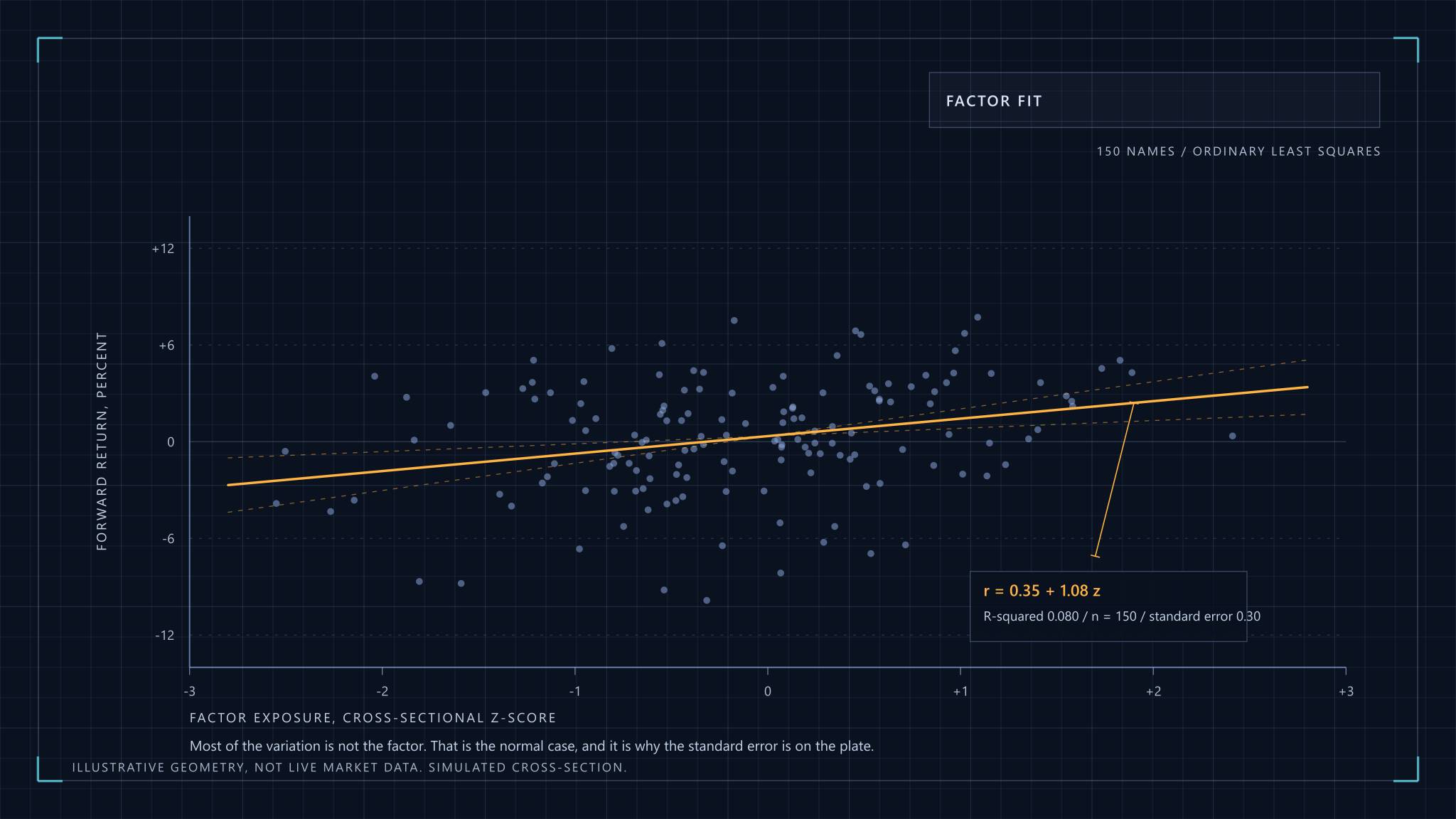
The standard formalisation is the work of Engle and Granger (1987), who showed that non-stationary series can share a stable long-run relationship and that this relationship can be estimated and tested. For a pair, the Engle-Granger two-step procedure is the practical tool. First regress one price on the other; the slope is your hedge ratio and the residual is your spread. Then test the residual for a unit root, usually with an augmented Dickey-Fuller test. If you can reject the unit root, the spread behaves as though it is pulled back to a mean.
Two cautions belong here. The test is run on a residual that was itself fitted to the same data, so the usual critical values are too lenient and need the adjusted tables designed for this purpose. And the regression is not symmetric: putting A on the left gives a slightly different hedge ratio from putting B there. Neither is wrong, but a pair that passes in one direction and fails in the other deserves suspicion.
When there are more than two legs
The Johansen test generalises the idea to baskets. Instead of one regression, it examines a whole system of prices at once and counts how many independent stable combinations exist. With three assets there can be zero, one or two. The advantage over Engle-Granger is that it does not force you to choose a dependent variable and it can find several relationships together.
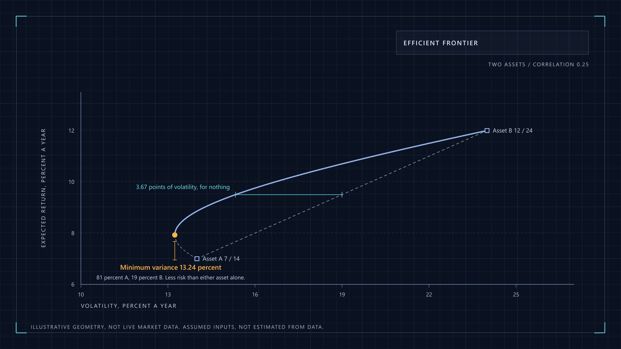
You do not need the mechanics to use the idea. What matters is the trade-off it exposes: a basket gives you more candidate spreads and more diversification across them, but every extra leg multiplies transaction costs and the number of ways the estimate can be fooled. For most individual practitioners, pairs and small baskets are the sensible limit.
A separate line of work builds the spread without picking partners at all. Avellaneda and Lee (2010) construct market-neutral portfolios by regressing stock returns on principal components or on sector ETFs and trading the residuals, and they also relate the strategy's performance to the market cycle. The point to take from it is that the "pair" is a special case of a general idea: strip out what the common factors explain, and trade what is left.
Where pairs come from
The original large-sample study, Gatev, Goetzmann and Rouwenhorst (2006), matched US stocks into pairs by minimum distance between normalised price series over a formation period, then traded divergences over the following months. Their sample runs on daily data from 1962 to 2002 and reports annualised excess returns of up to about 11 percent for self-financing portfolios of top pairs. That is a historical result for one rule on one market, in a period when the strategy was far less crowded, and it should be read that way.
A distance rule finds pairs that moved together. It does not find pairs that have a reason to. My preference is to start from the economics and then confirm with the statistics: two instruments that share a driver, such as two companies in the same line of business, two futures on neighbouring maturities, or an index and a basket that mostly replicates it. A pair found only by searching ten thousand combinations will contain plenty that pass a cointegration test by luck, and the more combinations you try, the more certain that becomes.
How fast does the spread come back
Passing a test says the spread reverts eventually. It does not say whether eventually means ten days or ten years, and that decides whether the pair is tradeable.
The usual model is the Ornstein-Uhlenbeck process, whose discrete form is simply an AR(1): each day the spread keeps a fraction phi of yesterday's deviation and receives a random shock. The half-life is the time for a deviation to shrink by half, which works out to the natural logarithm of 2 divided by minus the log of phi. You can estimate it by regressing the daily change in the spread on its lagged level.
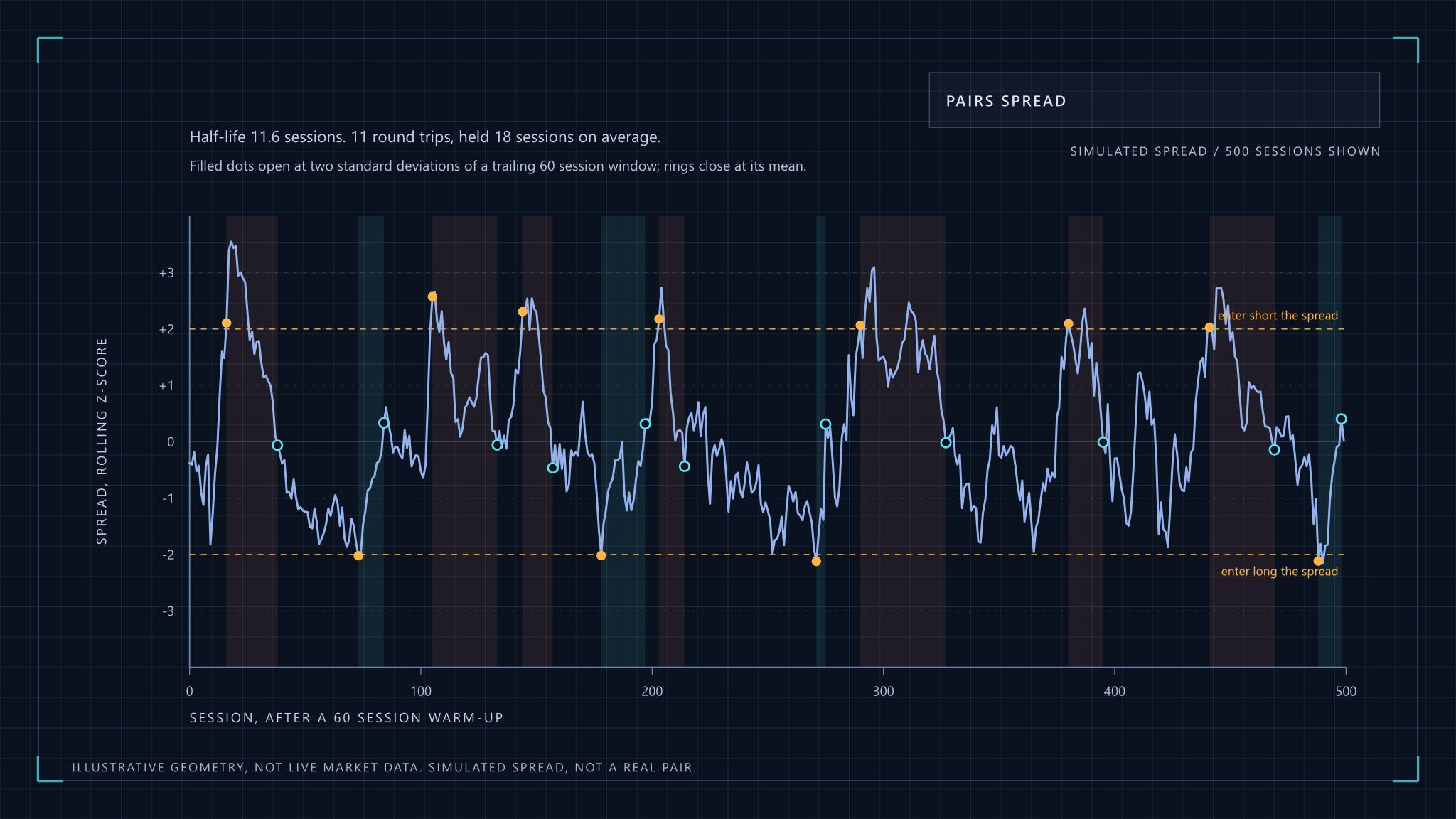
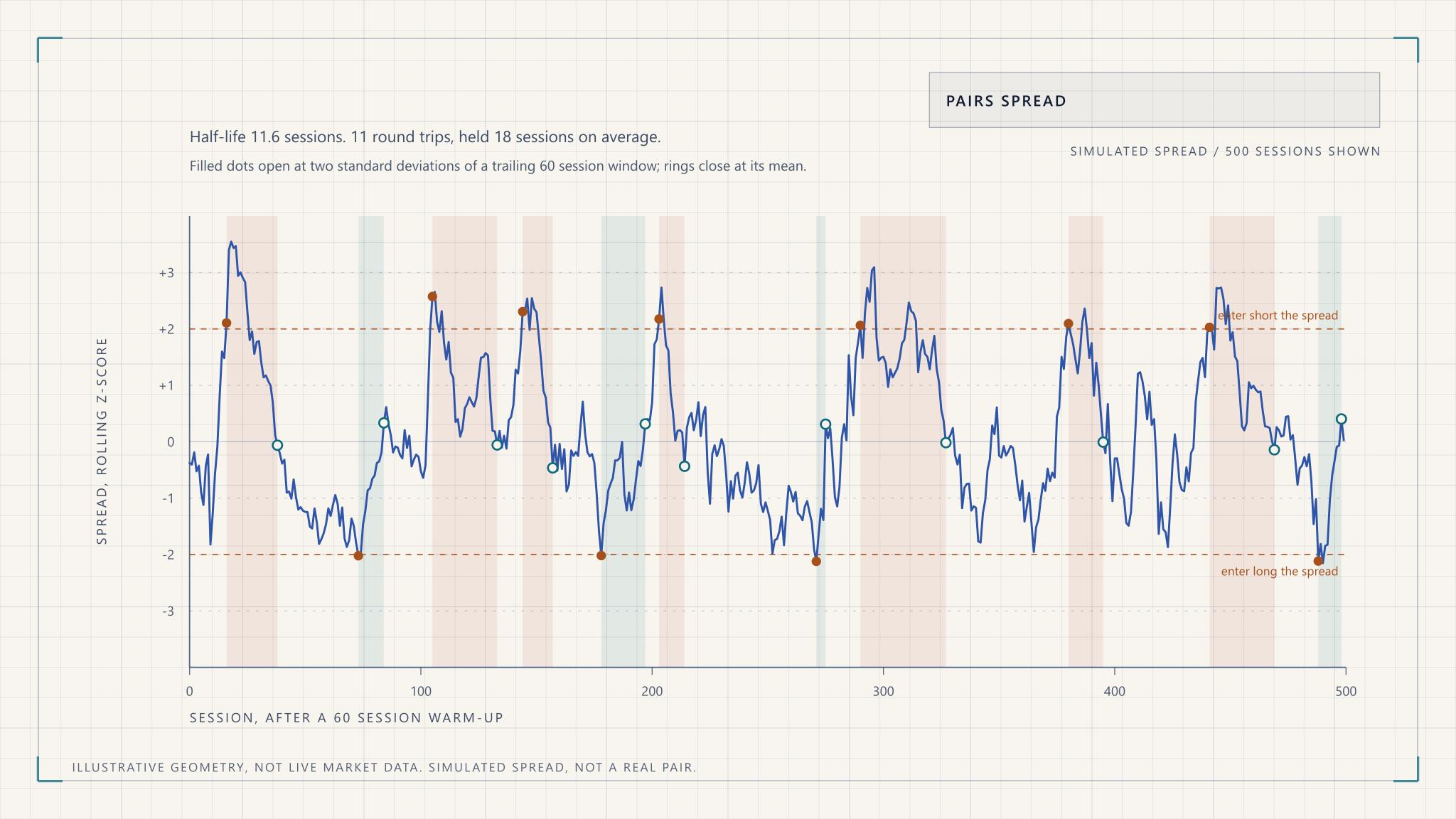
The simulated pair below uses a phi of 0.94, a true half-life of 11.2 days. A regression run on the 310 daily observations the simulation produced estimated 7.6 days. That is an error of about a third from roughly fifteen months of clean, perfectly stationary data, and real data is neither clean nor stationary.
Two practical rules follow. If the half-life is longer than the holding period you can tolerate, the pair is not for you regardless of its p-value. And treat any half-life estimate as a range, not a number, and re-estimate it on rolling windows to see how much it moves.
Entry thresholds are a cost decision
The usual rule is to enter when the z-score passes two in either direction and exit when it returns to zero. Two is a convention. What makes a threshold right or wrong is arithmetic about costs.
If you enter at a z-score of two and exit at zero, the gross move you are paid for is two standard deviations of the spread. A lower threshold trades more often and earns less per trade, while a higher one earns more per trade and trades rarely. Costs are paid per trade, so the question is how much of the gross each round trip surrenders.
| Entry z-score | Gross captured (spread sd of 1% of notional) | Share eaten by 0.4% round-trip costs |
|---|---|---|
| 1.0 | 1.0% | 40% |
| 1.5 | 1.5% | 27% |
| 2.0 | 2.0% | 20% |
| 2.5 | 2.5% | 16% |
Those figures are illustrative, not measured. The shape is what matters: at a z-score of one, nearly half of a perfectly executed trade is gone before slippage. A higher threshold looks safer on this arithmetic but has its own price, which is that fewer trades give you a thinner sample for judging whether the edge exists at all.
The exit deserves the same scrutiny. Waiting for exactly zero means holding through the slowest part of the reversion, where each extra day earns little. Some practitioners exit short of zero for that reason. The cost is that they leave some profit behind, and which side of that trade is better can only be settled with data on your own pair.
The short leg is where a market's rules show up
Everything above treats a short position as free and instant. It is neither. Short selling needs borrowable stock, borrowing has a fee that can change, the lender can recall the shares, and some markets restrict shorting outright.
As a worked example, take Indian cash equities. SEBI's framework for short selling (January 2024) does not permit naked short selling: every investor must deliver the securities sold at settlement. A short leg that is held for days, as a pair's usually is, therefore has to come from one of two places. The first is single-stock futures, where the short is a derivatives position with a lot size, an expiry, a basis to the cash price and a margin requirement under the exchange's SPAN framework (the NSE margin documentation is the authority). The second is the securities lending and borrowing mechanism run by NSE Clearing, where eligible securities, largely those in the futures and options segment, can be borrowed against a fee for a defined tenure.
Each choice reshapes the pair. Futures leave you trading a spread of a cash price against a futures price, so the roll at expiry becomes part of the trade and the basis becomes part of the spread. Borrowed stock keeps the legs in the same instrument but adds a fee that runs every day and the risk of an early recall that forces you out at a bad moment. Other markets have their own versions: locate requirements, short-sale bans in a crisis, borrow fees that spike on crowded names. The principle is portable. Before trusting a backtest, ask how the short leg would actually have been held, and whether it could have been held at all on the days that mattered. Rules and rates change, so check the current circulars rather than any summary, including this one.
What breaks the spread
Three failures account for most of the damage, and none of them shows up in an in-sample test.
Structural breaks. A merger, a change in a company's business, a regulatory change or a technology shift can permanently move the relationship between two prices. The spread then goes to four standard deviations and keeps going, and the rule that said to buy more at three is now averaging into a loss. This is why a hard stop on the z-score, set beyond where the relationship has plausibly ever gone, belongs in the rules from the start. A spread that is beyond its history is more likely to be broken than stretched.
Crowding. If many participants run similar spreads, entries and exits bunch together and the reversion that paid in the past gets arbitraged down. Worse, the crowd is hidden. You cannot see it in the data until it unwinds.
The unwind. The clearest case is August 2007. Khandani and Lo examined the week of 6 August 2007, when a number of quantitative long and short equity funds suffered unusual losses together, and argued that the evidence is consistent with a rapid liquidation of similar portfolios. They are open that their conclusions rest on indirect evidence and are speculative, and a reader should be equally careful. The lesson holds regardless of the exact cause. When one holder has to sell, the price move hurts every holder of the same position, so diversification across pairs offers little protection against a shared exit.
Sizing, and kill-switches that do not ask permission
A pair is a bet on a spread whose volatility is itself an estimate, so size by the spread's risk rather than by rupees. Dollar or rupee neutrality is a starting point: it makes the two legs equal in value, not equal in risk, and the hedge ratio from the regression is the better guide to how much of each to hold. Check it again at intervals, since it drifts. The ideas in risk management on volatility targeting apply directly, as does the point that estimates of volatility lag behind volatility itself.
Across a book of pairs, the dangerous number is the correlation between the spreads, not between the stocks. Twenty pairs that all depend on the same sector or the same funding conditions are one position. The treatment of concentration in portfolio construction is the right frame: measure risk contribution, not count.
Then there are the controls that act without a decision from you. A stop at a fixed z-score beyond history. A time stop, which closes the trade when it has lasted several half-lives with no reversion, since a trade that has not worked in that time is telling you the model is wrong. A portfolio-level loss limit that flattens everything. These are worth writing down before the first trade because the moment they are needed is the moment judgement is at its worst.
Testing without fooling yourself
A backtest of a pairs strategy is unusually easy to get wrong, because the whole method begins with a search. You search for pairs, then for thresholds, then for windows, and each search selects whatever happened to fit the sample. The result looks like skill and is mostly the search.
The safeguards are dull and effective. Select pairs and fit hedge ratios only on data that comes before the period you trade. Hold out a final stretch that you touch once, after every decision is made. Use walk-forward testing, where you re-estimate on a rolling window and trade the next block, so the test reproduces what you would actually have known at the time. Count every pair and parameter you tried, and treat a good result among thousands of candidates with the scepticism it deserves. The broader reasoning on this, including leakage and multiple testing, is in quantitative analysis.
Then put costs in properly: both the fee schedule and a slippage assumption set from the actual spread between bid and offer, plus the borrow or futures cost on the short leg. A strategy that survives all of this has earned a small amount of trust, no more. It still has to survive the day the relationship changes, and no test can tell you when that is.
Statistical Arbitrage and Pairs Trading