Combining RSI and MACD does not give you two independent confirmations. It gives you one rule with more parameters, which is easier to overfit and harder to believe. Whether the pairing adds anything real is an empirical question, and the honest way to answer it is to test the rule on data it was not fitted to, after costs, while counting how many rules you tried on the way.
That is a less exciting claim than the usual pitch, which says momentum and trend signals "confirm" each other. Sometimes they do. This article covers how each indicator is actually calculated, what the pairing can plausibly add, and the testing discipline that separates a finding from a story. The groundwork on treating indicators as testable claims is in an introduction to technical analysis, and this piece builds on it.
Every number below that comes from a simulation is labelled as one. Where Indian markets appear, they are a worked example of a principle that holds in any market.
What the two indicators actually compute
RSI and MACD both smooth price, and they differ in what they do with the smoothed result. Seeing that clearly is most of the battle.
RSI is a bounded ratio of recent gains to recent losses. J. Welles Wilder introduced it in his 1978 book, New Concepts in Technical Trading Systems, along with the 14-period default and the 70 and 30 reference levels. The calculation takes the average gain and the average loss over 14 periods, then forms 100 minus 100 divided by one plus their ratio. The detail that matters is the smoothing. After the first 14 periods Wilder does not use a simple moving window. He updates each average as the previous average times 13, plus today's value, all divided by 14. That is an exponential average with a weight of one-fourteenth, and it means an old shock never fully leaves the number.
MACD is the gap between two exponential moving averages of price, usually 12 and 26 periods, which Gerald Appel developed. A third exponential average of that gap, over 9 periods, is the signal line, and the histogram is the difference between the two. MACD is unbounded and carries the units of price, so a MACD reading on one index cannot be compared with one on another.
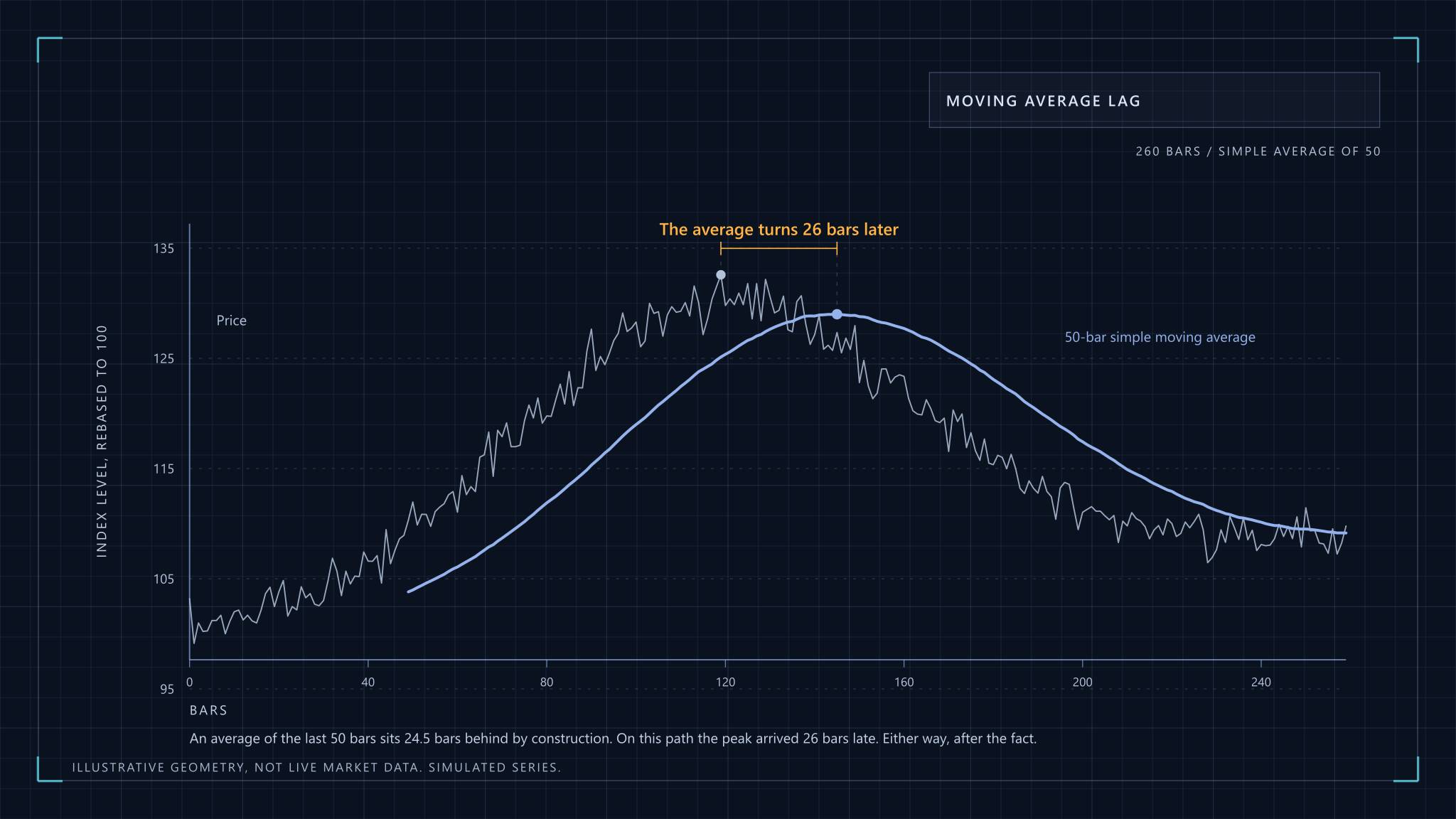
Two practical consequences follow. First, implementations disagree at the start of a series, because they seed the first average differently (a simple average, or just the first value). The disagreement fades after a few dozen bars, but it is why two charting platforms can show slightly different crossover dates. Second, both indicators are smoothing filters with a lag. A crossover tells you a move has already lasted long enough to shift an average. It describes the recent past and forecasts nothing.
One reads mean reversion, the other reads trend
The reason people pair them is sound in outline. RSI treats a sharp fall as a stretch that tends to snap back, so a rise through 30 is read as the stretch ending. MACD treats a crossover as evidence that a trend has started, so it is a follow-through signal. The pairing says: buy when a stretched market has begun to turn and the turn has some trend behind it.
The trouble is that these two readings disagree about what the market is doing. Mean reversion bets that the last move will reverse. Trend following bets that it will continue. Which one is right depends on the regime, and neither indicator tells you the regime. In a trending market, RSI sits above 70 for long stretches and a "sell above 70" rule fights the trend. In a range, MACD whipsaws, crossing back and forth around zero and charging costs each time.
So what does confluence buy? It reduces the number of signals, because requiring two events to coincide is a filter, and fewer trades means lower costs. What it does not do is make the signals independent. Both indicators are built from the same closing prices, and a rise through 30 followed by a MACD cross is largely one price move seen through two filters. Treat the agreement as a stricter trigger, not as corroboration from a separate source.
My view, which the testing below is designed to check rather than assume: the filter effect is real, and most of the apparent edge in confluence rules comes from the freedom to choose the parameters, not from the pairing.
What a confluence rule looks like when it is written down
A rule you can test has no adjectives in it. Here is one, using the definitions above.
- Signal: the 14-period RSI crosses up through 30 on a bar, and the MACD(12,26,9) line crosses above its signal line on the same bar or within the two bars before it, or the other way round. The rule fires on whichever event arrives second, so it never uses a bar that has not happened yet.
- Entry: the next bar's open, never the close that produced the signal, since that price was only known after the bar ended.
- Exit: a fixed number of bars, or an opposite MACD cross, decided before looking at any results.
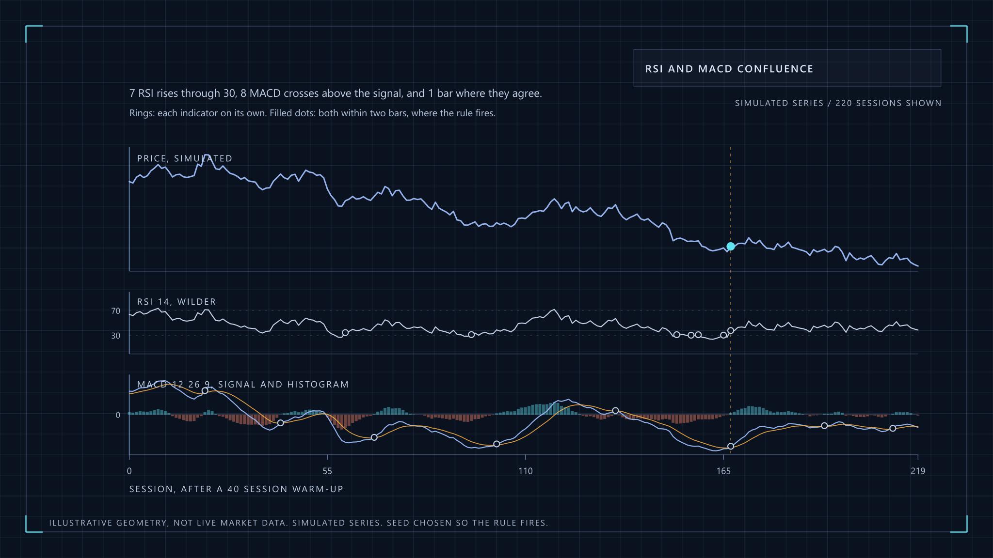
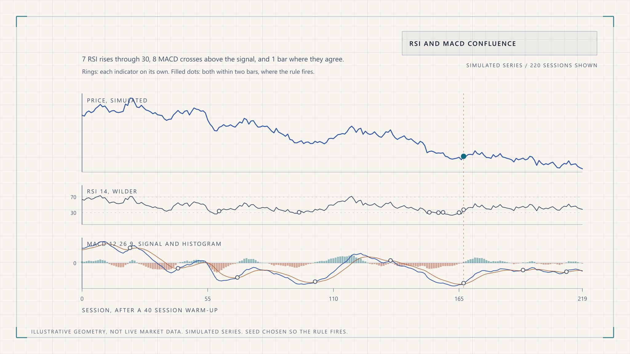
The figure shows that rule on a simulated series.
Notice that by the time the rule fires, RSI has already climbed to between 41 and 47, well away from the oversold zone. That is the lag showing. The second event to arrive is usually the MACD cross, and the oversold reading is several bars stale by then.
The statistical trap: more rules, more ways to be fooled
Every condition you add to a rule is another dial. An RSI level, an RSI period, a MACD speed, a window for how close the two events must be, an exit rule. Each has a plausible range, and the number of combinations multiplies. Run enough of them over a single history and some combination will look excellent, because chance alone supplies it.
Simulation makes this concrete. Take 2,000 simulated random walks of 250 bars each, where by construction there is nothing to find. The confluence rule above fires 0.78 times per path, a little under once a year. The mean log return over the five bars after those 1,514 signals was 0.021%, against 0.013% for an arbitrary bar, and the t-statistic of the difference is 0.36. The rule does nothing on noise, which is the correct answer.
Now do what an enthusiastic backtester does. Take 200 further random-walk paths of 1,500 bars, about six years of daily data, and a family of rules: RSI crosses up through a level between 20 and 40, with a period between 5 and 30, held for five bars. A single randomly chosen rule has a median annualised Sharpe ratio of -0.06 before costs, which is zero within noise. The best of 100 randomly chosen variants has a median of 0.74. That is a respectable-looking Sharpe ratio produced by selection alone, on data with no signal in it.
The academic literature says the same thing in more rigorous form. Brock, Lakonishok and LeBaron's 1992 study in the Journal of Finance tested moving-average and trading-range rules on the Dow Jones index from 1897 to 1986 and reported returns that standard null models, including a random walk and GARCH variants, could not easily explain. That is why it is cited so often. Sullivan, Timmermann and White then revisited the question in Data-Snooping, Technical Trading Rule Performance, and the Bootstrap, applying a bootstrap correction across the whole universe of rules that could have been tried, not just the winner. Their point is that a best rule has to be judged against how many rules were searched, and that adjustment is what most retail backtests omit.
The same logic runs through the wider finance literature. Harvey, Liu and Zhu argue in ...and the Cross-Section of Expected Returns that, given how many factors have been tested, a new one should clear a t-statistic above 3.0 rather than the conventional 2.0. Technical rules are a smaller version of the same problem. If you tried twenty parameter sets, a result that is significant at the usual threshold is unsurprising, and the bar should be higher.
How to test a confluence rule honestly
Seven habits, most of which are about refusing to flatter yourself.
Fix the rule family before you look. Write down every parameter you will vary and its range, and keep a count. That count is the number you need later to discount the best result. If you cannot say how many variants you tried, you cannot correct for it.
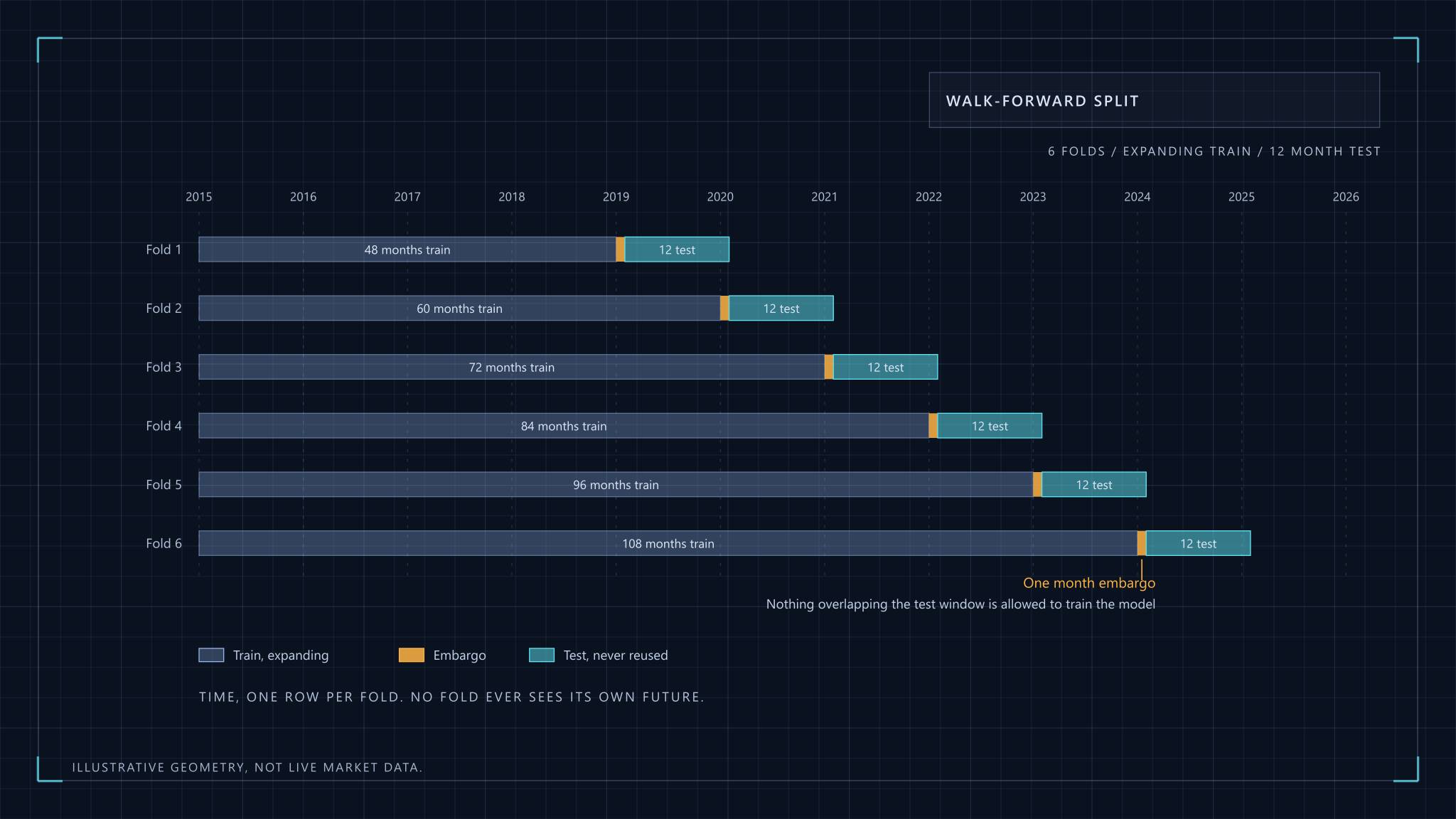
Use walk-forward validation. Choose parameters on one window, trade the next window untouched, then slide forward and repeat. The stitched out-of-sample results are the only equity curve worth looking at. The mechanics, including why shuffled cross-validation leaks information in time series, are covered in machine learning for stock selection, and they apply to a two-indicator rule exactly as they do to a model.
Hold out a final period you touch once. Walk-forward windows get reused as you iterate, so they slowly stop being out of sample. A last block of data, looked at a single time, is the only clean test. If the result disappoints, the honest move is to drop the rule, not to adjust it and look again.
Subtract realistic costs. This is where many technically plausible rules die. The next section works an example.
Count the trades. A rule that fires 0.78 times a year on one index gives roughly eight trades in a decade. That is an anecdote however it ended. Widen the universe, shorten the bar size, or accept that the data cannot answer the question.
Check stability across parameters. If RSI(14) works and RSI(12) and RSI(16) do not, you have found a quirk of the sample. A believable rule works across a neighbourhood of settings, modestly but consistently. A sharp peak at one setting is a warning.
Compare against the boring alternative. Over the same period and after the same costs, did the rule beat simply holding the index? A signal that trades often to match a position you could have held for free has not earned its complexity.
For a formal treatment of how many tries a result can survive, Bailey, Borwein, Lopez de Prado and Zhu's The Probability of Backtest Overfitting proposes a way to estimate how likely it is that the best in-sample configuration underperforms the median out of sample. It is worth reading for the framing alone, even if you never implement the method.
What costs do to a short holding period
Costs depend on the market, so treat this as an illustration of method. On the National Stock Exchange of India, a delivery-based purchase and a delivery-based sale of equity shares each attract Securities Transaction Tax at 0.1 per cent of trade value, according to NSE's circular on STT rates. That circular is dated April 2023, so confirm the current schedule before relying on it. A round trip is therefore 0.2 per cent before brokerage, GST and stamp duty. The exchange's own transaction charge, in its 2023 revision, was in the region of ₹3 per lakh of traded value on each side in the cash segment. That is 0.003 per cent, small beside the tax.
Run that through a rule. If it makes twenty round trips a year, STT alone costs 4 per cent a year, before the other charges and before slippage. For a strategy whose gross edge is a couple of percentage points, that is the entire result. The STT circular also lists a far lower rate, 0.001 per cent on the sale of a unit of an equity-oriented fund on the exchange, which is one reason a rule applied to an index fund and the same rule applied to individual shares can look completely different after costs. In any market the exercise is identical: find the primary schedule of taxes and charges, multiply by turnover, and subtract.
Slippage is the cost nobody publishes a circular for. A backtest that fills at the signal bar's close assumes you could trade at a price that was only known after the bar ended. Fill at the next open, add a spread allowance, and then stress it by doubling the allowance to see whether the result survives.
Filters that help, and the ones that only look like they do
Two filters earn their place in a confluence rule because they address real mechanisms rather than the fit.
A volatility filter stands aside when conditions are unusual. An oscillator level like 30 means something different when daily moves are twice their normal size, because a "stretched" reading is then ordinary. India VIX is one example of a volatility gauge you could condition on, and implied or realised volatility in any market works the same way. What matters is discipline: choose a rule such as "above the 80th percentile of trailing history", fix it, and do not tune it to rescue a bad year.
A liquidity floor excludes instruments where a handful of trades set the price. Indicator patterns on thin series are often patterns in the spread. Set a minimum average daily traded value, and make sure your own position is a negligible part of it.
The filters that look useful and mostly are not are the third and fourth indicators added "for extra confirmation". Each is a new dial, and as the simulation showed, dials are what the data rewards you for turning.
Stops and position size with ATR
Average True Range, also from Wilder's 1978 book, measures how far a market typically moves in a bar. True range for a bar is the largest of the high minus the low, the high minus the previous close, and the previous close minus the low. ATR smooths it with the same one-fourteenth weighting as RSI. Because it is expressed in price units, it scales a stop to the market's current temperament.
Sizing from it is arithmetic. Suppose you risk 0.5 per cent of ₹10 lakh on a trade, which is ₹5,000, and place the stop two ATRs from entry. If the ATR is ₹40 per unit, the stop sits ₹80 away and the position is 5,000 divided by 80, about 62 units. When volatility doubles, the position halves on its own. The numbers are hypothetical, but the property is the point: the loss you accept is fixed in advance, whatever the market is doing. Risk management essentials explains why this matters more than signal quality.
The stop multiple is itself a parameter. Choose it before testing, and report results at the neighbouring multiples so a reader can see whether the answer depends on your choice.
What a believable result looks like
Real edges in public technical rules are small, noisy and fragile. A believable result has the properties in the left column below, and a too-good one fails several of them.
| Believable | Too good to trust |
|---|---|
| Modest after-cost return, with a wide confidence interval | Smooth equity curve with a steep slope |
| Many trades, across several market regimes | A dozen trades in a single trending year |
| Similar results across neighbouring parameters | One sharp optimum at an odd setting |
| Out-of-sample result somewhat worse than in-sample | Out-of-sample as good as in-sample, or better |
| Rule family recorded before the test | Rule found by searching, justified afterwards |
| Honest count of variants tried | "Only a few" with no list |
The fourth row surprises people. A rule whose out-of-sample performance matches its in-sample performance exactly is usually a sign the out-of-sample data was not clean, because a fitted rule should degrade at least a little on fresh data. A high Sharpe ratio that survives costs on a rule that trades often should raise your suspicion first and your confidence second.
None of this proves the pairing is useless. RSI and MACD together are a reasonable structure for a hypothesis, and a disciplined test might find a modest effect in some market. It should not be a reason to size up. For where such a signal sits alongside everything else you hold, see portfolio construction, and quantitative analysis covers the data hygiene that underlies every figure here.
This article is educational only. It is not investment advice, it recommends no security, and the author is not a SEBI-registered Research Analyst or Investment Adviser. All price series shown are simulated.
RSI and MACD Confluence, Tested Honestly