Monte Carlo Value-at-Risk generates thousands of possible next-day market moves from an estimated joint distribution, revalues the portfolio under each one, and reads the loss threshold off the sorted results. It earns its extra cost in exactly two situations: the portfolio holds non-linear positions such as options, or you want to shock the inputs in ways history never did.
For a plain book of liquid linear holdings it adds little over the simpler methods, and it can add false confidence. This article builds the whole pipeline, shows where each stage quietly goes wrong, and ends with the question that matters more than the code: how would you know the number is any good?
All the numbers below come from simulated data with fixed random seeds, not from any market. The code and parameters are stated so that you can reproduce them. This is education, not advice, and it recommends no security.
Why simulate when historical and parametric VaR exist
Historical VaR replays past returns through today's portfolio. Parametric VaR assumes a normal distribution and multiplies volatility by a constant. Monte Carlo draws new scenarios from a model you choose, so it can price non-linear positions properly and can be bent to scenarios the past does not contain.
The three methods are set side by side in Risk Management Essentials, so the comparison is not repeated here. What matters is the trade each one makes. Historical VaR has no model but only as many tail observations as history happened to supply: 500 days of data give you five observations beyond the 99 percent line. Parametric VaR has a clean formula but cannot see an option's curvature. Monte Carlo can see the curvature and can generate a million tail observations, but only from the distribution you assumed. More paths reduce sampling noise. They do nothing about model error, and confusing the two is the most common mistake in this area.
My view is that a simulation is worth building when you can name the specific thing it captures that the cheaper method cannot. "It is more sophisticated" is not that thing.
Estimating the covariance matrix
The simulation is only as good as its covariance matrix. The two choices that matter are the estimation window and the weighting. A short equal-weighted window reacts fast but jumps when an old shock drops out. A long one is stable but slow to notice a regime change.
The standard compromise is the exponentially weighted moving average, popularised by the RiskMetrics system. Each day the new covariance is the old one multiplied by a decay factor lambda, plus the latest cross-product of returns multiplied by one minus lambda. The RiskMetrics Technical Document (J.P. Morgan and Reuters, 1996) uses 0.94 for daily trading horizons and 0.97 for longer investing horizons.
Those numbers have a concrete meaning. With lambda at 0.94, an observation's weight halves roughly every 11.2 days, and the most recent 20 days carry 71 percent of the total weight. Move lambda to 0.99 and you are close to a long equal-weighted window again, with the lag that implies. There is no correct decay, only a trade between responsiveness and noise, and it is worth checking how much your VaR moves when you change it. If a sensible change from 0.94 to 0.97 shifts the answer materially, that sensitivity is itself a finding.
Two further hazards sit here. A covariance matrix estimated from fewer observations than assets is not reliably positive definite, which breaks the next step. And correlations estimated in calm periods are the least trustworthy numbers in the model, because they are about to be tested. This is the same point made in portfolio construction: diversification is measured in quiet markets and needed in loud ones.
Cholesky: turning independent noise into correlated shocks
A random number generator gives independent standard normal draws. Real risk factors move together. Cholesky factorisation finds a lower-triangular matrix L such that L multiplied by its own transpose equals the covariance matrix. Multiply a vector of independent draws by L and the result has exactly the covariance you estimated.
The worked example is deliberately small. Three risk factors: two equity indices with daily volatility of 1.1 percent and 1.4 percent and a correlation of 0.65, plus a bond-like factor with 0.4 percent daily volatility and correlations of 0.10 and 0.05 to the two indices. The portfolio puts 50, 30 and 20 percent in them. Its daily volatility comes out at 0.89 percent. That is the number a parametric method would multiply by 2.326 to get a 99 percent VaR of 2.08 percent, and the simulation should land on the same figure when the shocks are normal. It does, which is a useful sanity check before anything cleverer is attempted.
import numpy as np

rng = np.random.default_rng(20250606)
vol = np.array([0.011, 0.014, 0.004])
corr = np.array([[1.00, 0.65, 0.10],
                 [0.65, 1.00, 0.05],
                 [0.10, 0.05, 1.00]])
cov = np.outer(vol, vol) * corr
w = np.array([0.5, 0.3, 0.2])

L = np.linalg.cholesky(cov)          # fails if cov is not positive definite
z = rng.standard_normal((10_000, 3))
returns = z @ L.T                    # correlated one-day factor returns
pnl = returns @ w                    # linear portfolio; revalue fully if not

var99 = -np.quantile(pnl, 0.01)
es99 = -pnl[pnl <= -var99].mean()
Revaluing the portfolio, which is the whole point
Once each scenario gives a set of factor moves, you reprice every position at the new levels. For shares and index funds this is just a weighted sum. For options it is a full pricing call per position per scenario, and that is the reason Monte Carlo exists.
A short at-the-money straddle shows why. Take an index option position, 30 days from expiry, 16 percent implied volatility, premium of 3.66 per 100 of index level, and simulate the index with 1.1 percent daily volatility. At the money, the net delta is about 0.018, so a delta-normal VaR reports 0.05 per 100: the position looks nearly riskless. Revalue every scenario with the Black-Scholes formula one day later and the 99 percent VaR is 0.63, with expected shortfall of 0.81. That is more than ten times the linear answer, and the whole of the difference is gamma. Volatility is held constant in that run. Let implied volatility rise with a falling index, as it does, and the real loss is larger again.
This is the use case that justifies the machinery. A defined-risk structure such as the butterflies covered here has a bounded loss that you can read off a payoff diagram, so simulation adds little. A short straddle has a loss that grows faster than the move, and no first-order approximation will describe it. Pricing it correctly in every scenario is also the honest basis for deciding how much hedging is needed, a question taken up in hedging a portfolio with index options.
The cost is real. Ten thousand scenarios across a few thousand positions is tens of millions of pricing calls, which is why production systems approximate with Greeks for most positions and fully revalue only the awkward ones.
Reading VaR and expected shortfall off the distribution
Sort the simulated profit and loss from worst to best. The 99 percent VaR is the loss at the one-percent mark. Expected shortfall is the average of every loss beyond that mark. There is no formula to apply: both are counting exercises on the sorted list.
The gap between 2.08 and 2.32 is small, because a normal tail is thin and there is not much beyond the threshold. The gap between 2.44 and 3.29 is large. That difference in how bad the bad days are, given identical volatility, is invisible to VaR alone and is the case for looking at both numbers.
Fat tails, and why normal shocks flatter you
Normal shocks make extreme days far too rare. Daily returns in most markets show excess kurtosis, meaning more very large and very small moves than a bell curve allows. Draw shocks from a Student-t distribution, or resample actual standardised residuals, and the simulated tail thickens to something closer to what markets do.
Scaling matters here. A t distribution with 4 degrees of freedom has more variance than a standard normal, so the draws must be rescaled to unit variance, or you have changed the volatility and the tail at once and learned nothing about either. The degrees of freedom are an input to be estimated and judged, and 4 is deliberately harsh.
| Confidence | VaR, normal | ES, normal | VaR, t (4 d.f.) | ES, t (4 d.f.) |
|---|---|---|---|---|
| 95% | 1.47% | 1.84% | 1.37% | 2.01% |
| 97.5% | 1.75% | 2.09% | 1.76% | 2.47% |
| 99% | 2.08% | 2.38% | 2.32% | 3.19% |
| 99.9% | 2.76% | 2.99% | 4.34% | 5.95% |
Each column comes from 400,000 simulated paths, so sampling noise is small. Two features deserve attention. At 95 percent the t distribution gives a lower VaR than the normal, because with the same variance it puts more mass in the very centre and in the far tails and less in the shoulders. And the divergence accelerates with confidence: at 99.9 percent the t answer is more than half as large again as the normal one.
One caveat on the construction. The t shocks were drawn independently for each factor and then mixed by the Cholesky matrix. That dilutes joint extremes, so real markets, where everything falls on the same day, are rougher than this. A multivariate t with one shared scaling draw would give heavier joint tails still.
How many paths are enough
Sampling error in a tail quantile shrinks with the square root of the number of paths, and it is larger in the tail than at the median because few paths land there. At 10,000 paths a 99 percent VaR carries a standard error of about 1.5 percent of its own value. At 1,000 paths it is about 5 percent.
The standard error of a quantile is the square root of p times (1 minus p) divided by n, all divided by the density at the quantile. The density term is small in the tail, which is why tails need more paths than centres do.
Two readings follow. To halve the error you need four times the paths, so the returns diminish quickly, and variance reduction techniques such as antithetic draws or importance sampling are worth more than brute force once you are past a hundred thousand. And the fat-tailed run in the figure earlier gave a 99 percent VaR of 2.44 percent at 10,000 paths while the 400,000-path version gave 2.32 percent. Heavy tails make the quantile noisier for the same path count, so a number that looks stable under normal shocks may not be under t shocks.
Stress testing the inputs
A stress test changes the inputs, not just the draws. Raise every volatility by a stated factor, push the correlations toward one, or add a fixed jump to a factor, and rerun. The point is to find the inputs the portfolio is secretly most sensitive to. With normal shocks the stressed figures also have a closed form, so the simulation can be checked against it.
Try it on the three-factor example. Pushing the correlation between the two equity indices from 0.65 to 0.95 and the bond factor's correlation to both from near zero to 0.6 lifts the 99 percent VaR from 2.08 to 2.35 percent, a rise of 13 percent. Scaling every volatility by 1.5 lifts it to 3.12 percent. Doing both gives 3.52 percent. The honest reading is that volatility dominates here, because the book is mostly equity and the equity correlation was already high. The correlation stress bites through the bond holding, whose diversification benefit was the part borrowed from calm periods. Which stress matters depends on where your diversification actually sits, and a stress run is how you find out.
Reverse stress testing runs the other way. Instead of choosing a scenario and reading the loss, choose a loss you could not survive and search for the combination of moves that produces it, then ask whether that combination is as implausible as you hoped.
Stress results are not probabilities. A stressed VaR is a statement of the form "if this happened, then", and the discipline is to resist attaching a likelihood to it.
Backtesting: does the number deserve trust
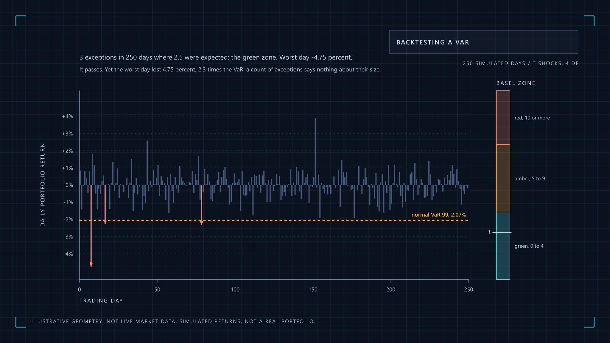
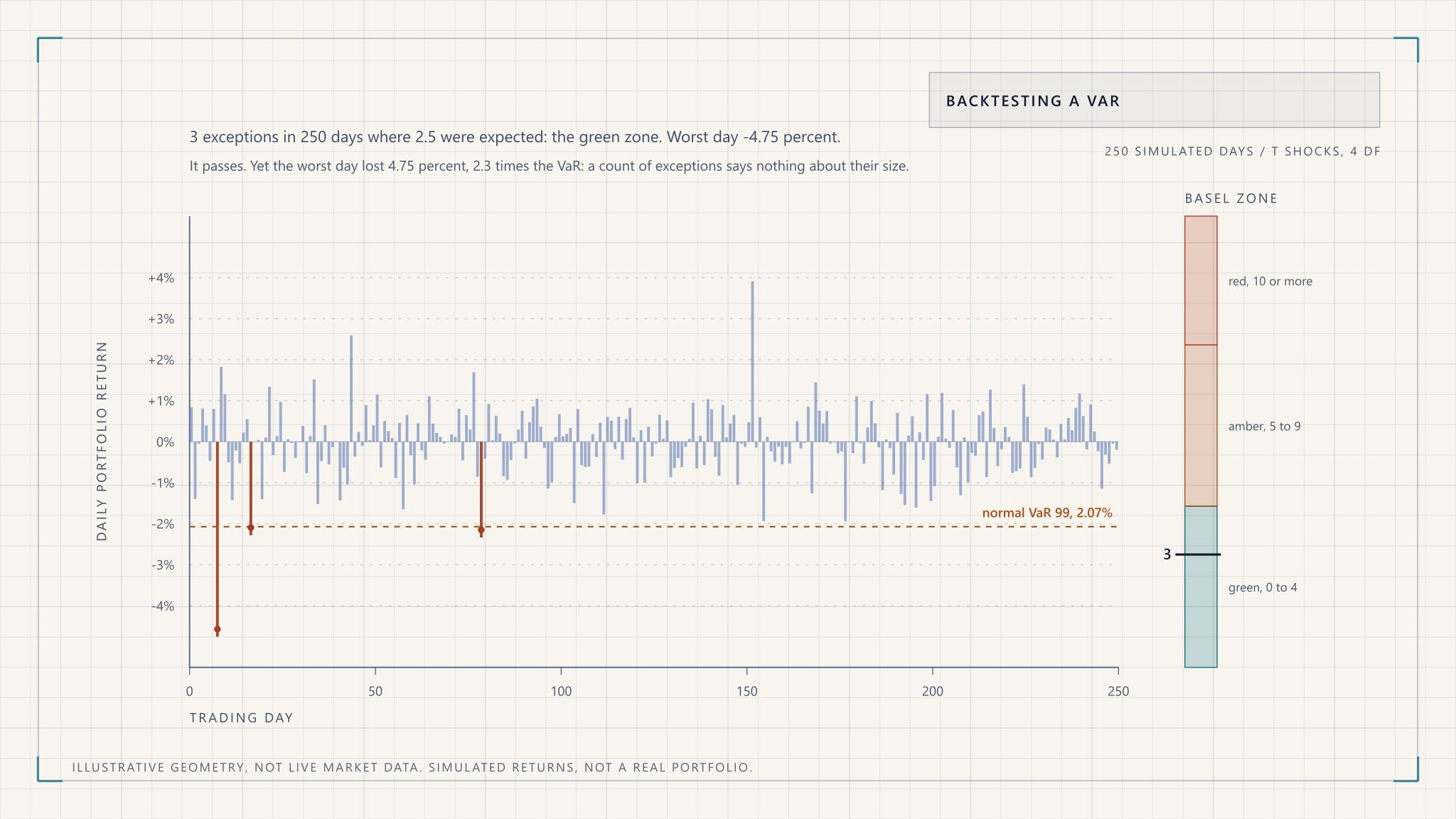
A VaR model makes a testable claim: a 99 percent one-day VaR should be exceeded on about 1 day in 100. Count the exceptions over a year and compare with the 2.5 expected in 250 days. Kupiec's proportion-of-failures test turns that count into a formal accept or reject.
The test statistic is a likelihood ratio compared with a chi-squared distribution with one degree of freedom, whose 5 percent critical value is 3.84. Kupiec's 1995 paper, Techniques for Verifying the Accuracy of Risk Measurement Models, introduced it. Over 250 days at 99 percent, the arithmetic gives these results: 5 exceptions score 1.96 and pass, 6 score 3.56 and still pass, 7 score 5.50 and fail. Zero exceptions score 5.03 and also fail, because a model that never breaches is too conservative and is tying up capital for nothing.
The weakness is power. With one year of data the test cannot tell a good 99 percent model from one that is wrong by a factor of two in exceedance rate until the damage is plain, and it says nothing about whether exceptions cluster, which is the more dangerous failure. A model with a few exceptions all in the same fortnight has failed in a way the count hides.
Regulators use a simpler device. The Basel framework's backtesting rules, in MAR32 of the Basel Framework, sort a 250-day sample into zones: green for 0 to 4 exceptions, amber for 5 to 9, red for 10 or more, with the backtesting multiplier rising from 1.50 in the green zone to 2.00 in the red. The amber zone begins where the binomial probability of seeing that many exceptions or fewer from an accurate model reaches 95 percent, which is why 5 is the boundary. The red zone is where that probability passes 99.99 percent, so an accurate model almost never lands there. It is a statistical decision rule with a penalty attached, and it is worth reading as one.
From VaR to expected shortfall
VaR gives a threshold and ignores what lies beyond it. Expected shortfall averages the tail, and unlike VaR it never penalises diversification. That is why the Basel Committee replaced 99 percent VaR with expected shortfall at 97.5 percent for the trading book's internal models approach.
The theoretical argument is from Artzner, Delbaen, Eber and Heath, whose paper Coherent Measures of Risk (Mathematical Finance, 1999) lists the properties a sensible risk measure should have, one of which is subadditivity: combining portfolios should never increase measured risk. VaR can violate it. They also suggest tail conditional expectation as a coherent alternative, which is close to what is now called expected shortfall.
The regulatory text is direct: under MAR33.3, "in calculating ES, a bank must use a 97.5th percentile, one-tailed confidence level." The two choices of 99 and 97.5 were set to look similar, and under normality they are: in the table above, normal expected shortfall at 97.5 percent is 2.09 percent against a 99 percent VaR of 2.08. Under fat tails they separate, with the t-shock expected shortfall at 97.5 percent at 2.47 percent against a VaR of 2.32 percent. The switch made the number respond to tail shape, which was the aim.
Expected shortfall is not free of problems. It is harder to backtest, since a single exceedance count no longer tests it directly, and the Basel framework still backtests with VaR at both the 99th and 97.5th percentiles for that reason. It is also more sensitive to the tail model than VaR is, which makes the fat-tail choices above matter more, not less.
One worked example from exchange practice
Risk-based margining is the everyday version of all this. As one example from a single market, SEBI's discussion paper on risk management for the cash market describes a VaR margin intended to cover the largest loss expected on 99 percent of days. Liquid securities are margined on one-day losses and illiquid ones on three-day losses, scaled by the square root of three, and volatility is estimated with an exponentially weighted moving average of daily returns.
That is the pipeline above in miniature: a decay-weighted volatility, a 99 percent threshold, and a horizon scaled to liquidity. The parameters and categories have been revised several times since that paper, so read the current NSE and SEBI circulars rather than relying on any description of the rates, including this one. The method carries over to any market with an exchange margining system.
What the number still cannot tell you
A Monte Carlo VaR is a statement about the model, conditional on its inputs, over a short horizon in orderly markets. It does not capture liquidity that vanishes, a position you cannot exit in the assumed horizon, or a correlation structure that did not exist in your window. All three are worth stating next to the number whenever it is reported.
The sensible way to use it is as one of several views: the simulated VaR and expected shortfall, the same figures under stressed inputs, and the backtest record. If they disagree, trust the disagreement. For a wider view of sizing, drawdowns and the controls that make limits stick, return to risk management essentials, and for the habit of checking whether a clean backtest means anything at all, quantitative analysis in finance covers it.
Monte Carlo Value-at-Risk, Step by Step